
ESG评分多空投资策略:买ESG评分高的公司真的能赚钱吗?(附分层回测通用代码)

1.前言
前情提要
结论先行:
本文对华证与 Wind 的 ESG 评分分别构建“按披露日横截面分层、T+1 生效、前向填充到日频、等权持有到下一次披露”的策略框架,在最长可追溯样本期内进行系统回测。回测结果如下:
进攻性弱:ESG高分≠更高收益。在完整的牛熊与震荡周期中,多数时段无法创造超额回报。
防守性强:优势在于显著降低波动与回撤,扮演“风险减震器”的角色。
行情有阶段:有效性高度依赖市场环境,仅在2019-2021等特定窗口期表现突出。
数据源:华证 ESG(综合/E/S/G 分项)、Wind ESG(综合)。两家机构分别回测。
样本频率:ESG 为季度披露,日线行情为日度
有效区间:
Wind ESG:2018-2023
华证 ESG:2008-2023
日线行情覆盖:2008-2023
去极值与清洗:日收益按分位截尾处理(默认 0.5%/99.5%),剔除异常与 ST。
wind与华证ESG数据均为评分格式,我们可以很轻松地对评分进行分层,因此我们将数据格式统一后可以直接调用函数针对不同来源的分数进行相同的分层处理。
tip
通过Quantide Research平台,运行下列代码可实现数据预下载:
import pandas as pd
import os
start = datetime.date(2009, 1, 1)
end = datetime.date(2023, 12, 29)
universe = -1
#获取所有股票
df = load_bars(start, end,-1)
df.to_parquet('daily_data.parquet')
下载到的数据格式如下:
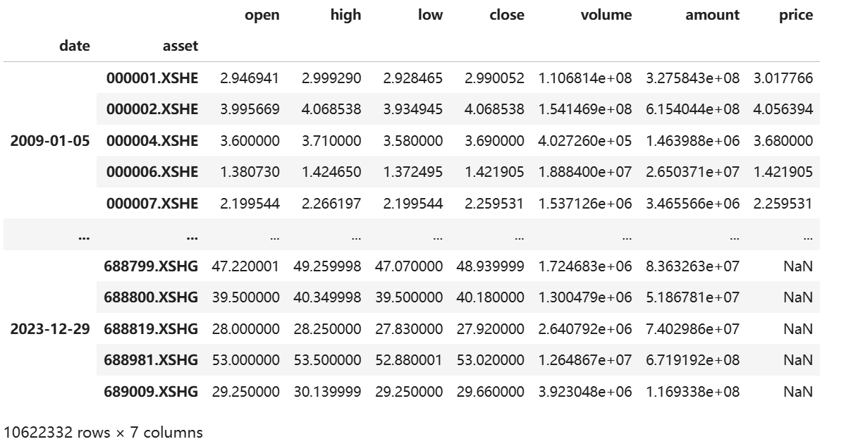
从返回结果中我们能看到,研究平台数据非常齐全,每个股票的交易量、交易金额等指标均有记录,其他的日线策略回测我们也可以采取该数据。
attention
有了研究数据,接下来我们实现ESG分层收益分析。
2.分析步骤
attention
首先,我们需要先导入分析所需要的库
import pandas as pd
import numpy as np
import matplotlib.pyplot as plt
import quantstats as qs
import os
from datetime import datetime
import warnings
qs.extend_pandas()
warnings.filterwarnings('ignore')
plt.rcParams['font.family'] = 'WenQuanYi Zen Hei'
import matplotlib as mpl
plt.rcParams['font.sans-serif'].insert(0, 'DejaVu Sans')  # 优先使用DejaVu Sans
# 创建图表输出目录
if not os.path.exists(str(get_jupyter_root_dir() / "reports/ESG/")):
    os.makedirs(str(get_jupyter_root_dir() / "reports/ESG/"))

report_dir = str(get_jupyter_root_dir() / "reports/ESG/")
2.1数据清理
- 读取华证和 Wind 的 ESG 数据以及全市场日线数据。
- 剔除 ST 股票、异常日期和空值,保留必要字段(股票代码、日期、评分),按日期和股票排序。
def preprocess_esg_data(esg_data, score_column, exclude_st=True):
    """预处理ESG数据,统一列名和格式,可选剔除ST股票"""
    df = esg_data.copy()

    # 统一重命名:使用列索引重命名(两个数据源格式已统一)
    df = df.rename(columns={
        df.columns[0]: 'stock_code',  # 证券代码
        df.columns[1]: 'stock_name',  # 证券名称
        df.columns[2]: 'date'         # 日期(无论是"评级日期"还是"交易日期")
    })
    # 处理日期列,过滤无效日期
    df['date'] = pd.to_datetime(df['date'], errors='coerce')
    df = df.dropna(subset=['date'])
    # 剔除ST股票(如果启用)
    if exclude_st and 'stock_name' in df.columns:
        st_mask = df['stock_name'].str.contains('ST', na=False)
        st_count = st_mask.sum()
        if st_count > 0:
            df = df[~st_mask]
            print(f"[INFO] 剔除ST股票:{st_count:,} 条记录")
    # 保留必要的列
    keep_cols = ['stock_code', 'date', score_column]
    df = df[keep_cols]
    df = df.dropna(subset=[score_column])
    df = df.sort_values(['date', 'stock_code'])
    print(f"[OK] 数据预处理完成,共 {len(df):,} 条记录")
    print(f"  日期范围:{df['date'].min().strftime('%Y-%m-%d')} 至 {df['date'].max().strftime('%Y-%m-%d')}")
    print(f"  股票数量:{df['stock_code'].nunique():,}")
    return df


wind_esg_data = pd.read_parquet('wind_esg.parquet')
esg_wind = preprocess_esg_data(wind_esg_data, score_column='WindESG评级')
2.2评分分层
- 对每个披露日的 ESG 得分进行横截面排序并分层。
- 层数可调(默认 10 层),第 1 层为最低评分的 10%,第 10 层为最高评分的 10%。
该过程会分别对华证综合得分、E/S/G 子项得分以及 Wind ESG 评级独立执行。
def classify_score_per_period(esg_df, score_column, n_layers=5, data_source='wind'):
    """统一的评分分层函数(支持华政和Wind)"""
    df = esg_df.copy().sort_values(['date','stock_code'])

    def _cut_period(g):
        # 对每个披露日期的截面数据分层(robust to ties)
        try:
            g['layer'] = pd.qcut(
                g[score_column].rank(method='first'),
                q=n_layers, labels=False, duplicates='drop'
            ) + 1
        except Exception:
            ranks = g[score_column].rank(method='first')
            g['layer'] = pd.cut(ranks, bins=n_layers, labels=False, include_lowest=True) + 1
        return g

    df = df.groupby('date', group_keys=False).apply(_cut_period)

    print(f"[OK] {data_source}评分分层完成(每个披露日截面分{n_layers}层)")
    print(f"各层总体分布:")
    layer_dist = df.groupby('layer').size()
    for layer, count in layer_dist.items():
        print(f"  Layer {layer}: {count:,} ({count/len(df)*100:.1f}%)")

    return df[['stock_code','date','layer']]

esg_wind_classified = classify_score_per_period(esg_wind, 'WindESG评级', n_layers=10, data_source='Wind')
2.3日度收益率计算
从全市场日线行情中计算每只股票的日收益率,剔除异常值与极端涨跌(默认截尾 0.5% 分位)。确保样本干净,避免极端波动干扰层内均值。
daily_data = pd.read_parquet('daily_data.parquet')
def prepare_daily_returns(daily_df, price_col='close', min_price=0.01,winsor_p=0.005):
    """从日线数据中计算收益率(含清洗和去极值)"""
    print("正在准备日线收益率数据...")

    df = daily_df.reset_index().rename(columns={'asset': 'stock_code'})
    df['date'] = pd.to_datetime(df['date'])
    df = df[['stock_code','date',price_col]].copy()

    # 价格数值化与过滤:非正、极小值、缺失全滚粗
    df[price_col] = pd.to_numeric(df[price_col], errors='coerce')
    df = df.dropna(subset=[price_col])
    df = df[df[price_col] > min_price]

    df = df.sort_values(['stock_code','date'])
    ret = df.groupby('stock_code')[price_col].pct_change()

    # 干掉 inf/-inf、超大绝对值
    ret = ret.replace([np.inf, -np.inf], np.nan)

    lo = ret.quantile(winsor_p)
    hi = ret.quantile(1 - winsor_p)
    ret = ret.clip(lo, hi)

    df['return'] = ret
    df = df.dropna(subset=['return'])

    # 可选:把 |r|>30% 的样本数量打个日志
    outlier_cnt = (df['return'].abs() > 0.3).sum()
    if outlier_cnt > 0:
        print(f"[WARN] |return|>30% 样本: {outlier_cnt:,}")

    print(f"[OK] 日线数据处理完成,共 {len(df):,} 条记录")
    print(f"  股票数量:{df['stock_code'].nunique():,}")
    print(f"  平均日收益率:{df['return'].mean():.4%}")

    return df[['stock_code','date','return',price_col]]
daily_returns = prepare_daily_returns(daily_data)
2.4将评级扩展到日线
从季度到日度:三步法
截面分层:每个披露日内按分位切分为 N 层(本文用 10 层)。
分层标签从披露日向前持有,直到下一个披露日更新。
T+1 生效:为避免信息穿越,分层信号次一交易日才开始作用到收益。
将季度ESG 评级扩展到日度频率,并采用 T+1 生效机制(即评级在披露后一交易日才生效),保证信号和收益的时间顺序不被污染。即评级发布后第二天进行调仓。
def expand_to_daily_with_t1(esg_layers, daily_df):
    """将季度ESG评级扩展到日线,并实施T+1延迟"""
    print("正在将季度ESG数据扩展到日线(T+1延迟)...")

    # 统一股票代码格式
    def convert_stock_code(code):
        code = str(code)
        if code.endswith('.SZ'):
            return code.replace('.SZ', '.XSHE')
        elif code.endswith('.SH'):
            return code.replace('.SH', '.XSHG')
        return code

    esg = esg_layers[['stock_code','date','layer']].copy()
    esg['stock_code'] = esg['stock_code'].apply(convert_stock_code)
    esg['date'] = pd.to_datetime(esg['date'])

    dly = daily_df[['stock_code','date','return']].copy()
    dly['stock_code'] = dly['stock_code'].astype(str)
    dly['date'] = pd.to_datetime(dly['date'])

    # 合并
    merged = dly.merge(esg, on=['stock_code','date'], how='left')
    merged = merged.sort_values(['stock_code','date'])

    # 前向填充最新的layer
    merged['layer'] = merged.groupby('stock_code')['layer'].ffill()

    # T+1延迟:今天的收益使用昨天的layer
    merged['layer'] = merged.groupby('stock_code')['layer'].shift(1)

    merged = merged.dropna(subset=['layer'])
    merged['layer'] = merged['layer'].astype(int)

    print(f"[OK] 合并完成,共 {len(merged):,} 条记录(含T+1延迟)")

    return merged

daily_with_wind = expand_to_daily_with_t1(esg_wind_classified, daily_returns)
# 清洗
daily_with_wind = daily_with_wind.replace([np.inf, -np.inf], np.nan)
daily_with_wind = daily_with_wind[daily_with_wind['return'].between(-0.5, 0.5)]
print(f"[INFO] 清洗后Wind数据:{len(daily_with_wind):,} 条记录")
2.5分层回测
- 对每个交易日、每一层分别计算等权平均收益,过滤掉成分过少的层(默认 ≥10 支股票)。
- 利用QuantStats库快速计算各层与多空组合的主要绩效指标:年化收益、波动率、夏普比率、最大回撤、Calmar 比率、Sortino 比率、胜率等。
def backtest_hold_between_events(dly_with_layer, min_names_per_layer_day=10):
    """执行分层回测(使用quantstats简化指标计算)"""
    print("正在执行分层回测(使用quantstats)...")

    df = dly_with_layer.copy()

    # 诊断:层内日样本数分布
    print("层内日样本数分布:")
    print(df.groupby(['layer'])['date'].nunique().describe())
    print("单日层内成分数的分位:")
    print(df.groupby(['date','layer'])['stock_code'].nunique().quantile([.1,.25,.5,.75,.9]))

    # 先统计每天每层有多少只股票
    counts = df.groupby(['date','layer'])['stock_code'].nunique()

    # 仅保留成分数≥阈值的层日(避免"一只妖股带飞全层")
    valid = counts[counts >= min_names_per_layer_day].index
    df = df.set_index(['date','layer']).loc[valid].reset_index()

    print(f"[INFO] 过滤后保留 {len(df):,} 条记录(每层日至少{min_names_per_layer_day}只股票)")

    # 每日等权layer收益;空缺日留作NaN
    layer_daily = df.groupby(['date','layer'])['return'].mean().unstack()

    # 确保索引是DatetimeIndex
    if not isinstance(layer_daily.index, pd.DatetimeIndex):
        layer_daily.index = pd.to_datetime(layer_daily.index)

    # 对数收益率
    def _cumprod_stable(s):
        r = s.dropna()
        if len(r) == 0:
            return pd.Series(index=s.index)
        logcum = np.log1p(r).cumsum()
        cr = np.exp(logcum)
        return cr.reindex(s.index).ffill()

    cum = layer_daily.apply(_cumprod_stable)

    # ========== 使用quantstats计算各层统计指标(更简洁!)==========
    stats = {}
    for layer in layer_daily.columns:
        r = layer_daily[layer].dropna()
        if len(r) == 0:
            continue

        stats[f'Layer_{layer}'] = {
            'Total_Return': qs.stats.comp(r),
            'Annualized_Return': qs.stats.cagr(r),
            'Volatility': qs.stats.volatility(r),
            'Sharpe_Ratio': qs.stats.sharpe(r),
            'Max_Drawdown': qs.stats.max_drawdown(r),
            'Calmar_Ratio': qs.stats.calmar(r),
            'Sortino_Ratio': qs.stats.sortino(r),
            'Win_Rate': qs.stats.win_rate(r),
        }

    # 计算多空策略
    long_short_returns = None
    long_short_cumulative = None

    if len(layer_daily.columns) >= 2:
        top = layer_daily.columns.max()
        bot = layer_daily.columns.min()
        # 只在两层都有数据的日期计算多空
        r_ls = pd.concat([layer_daily[top], layer_daily[bot]], axis=1).dropna()
        ls = r_ls.iloc[:,0] - r_ls.iloc[:,1]
        long_short_returns = ls
        long_short_cumulative = (1 + ls).cumprod()

        # 使用quantstats计算多空策略指标
        stats['Long_Short'] = {
            'Total_Return': qs.stats.comp(ls),
            'Annualized_Return': qs.stats.cagr(ls),
            'Volatility': qs.stats.volatility(ls),
            'Sharpe_Ratio': qs.stats.sharpe(ls),
            'Max_Drawdown': qs.stats.max_drawdown(ls),
            'Calmar_Ratio': qs.stats.calmar(ls),
            'Sortino_Ratio': qs.stats.sortino(ls),
            'Win_Rate': qs.stats.win_rate(ls),
        }

    print("[OK] 回测完成!")

    return {
        'daily_returns': layer_daily,
        'cumulative_returns': cum,
        'statistics': stats,
        'long_short_returns': long_short_returns,
        'long_short_cumulative': long_short_cumulative
    }

#计算开始
wind_results = backtest_hold_between_events(daily_with_wind, min_names_per_layer_day=10)
print("\nWind评分回测结果:")
print(pd.DataFrame(wind_results['statistics']).T.to_string())
2.6 可视化与报告输出
使用QuanStats生成四类图表:
- 各层累计收益曲线
- 多空策略收益与回撤
- 核心绩效指标对比
- 指标汇总表格
# 保存结果
all_results = {}
all_results['Wind评分'] = wind_results

def plot_backtest_results(results, title='ESG_Backtest', save_path=f'{report_dir}'):
    """增强的可视化回测结果(使用quantstats风格)"""
    cumulative_returns = results['cumulative_returns']
    statistics = results['statistics']
    long_short_cumulative = results['long_short_cumulative']
    long_short_returns = results['long_short_returns']

    # 根据实际层数动态生成配色方案
    n_layers = len(cumulative_returns.columns)
    # 使用 tab20 配色方案支持更多层数,如果层数少用 Set2
    if n_layers <= 8:
        colors = plt.cm.Set2(np.linspace(0, 1, n_layers))
    else:
        colors = plt.cm.tab20(np.linspace(0, 1, n_layers))

    fig, axes = plt.subplots(2, 2, figsize=(18, 12))
    fig.patch.set_facecolor('white')

    # 1. 各层累计收益
    ax1 = axes[0,0]
    for i, layer in enumerate(cumulative_returns.columns):
        ax1.plot(cumulative_returns.index, cumulative_returns[layer],
                label=f'Layer {layer}', linewidth=2.5, color=colors[i], alpha=0.8)
    ax1.axhline(y=1, color='black', linestyle='--', alpha=0.3, linewidth=1)
    ax1.set_title('Cumulative Returns by Layer', fontsize=14, fontweight='bold', pad=15)
    ax1.set_xlabel('Date', fontsize=11)
    ax1.set_ylabel('Cumulative Return', fontsize=11)
    ax1.legend(loc='best', framealpha=0.9, fontsize=10)
    ax1.grid(True, alpha=0.3, linestyle=':', linewidth=0.5)
    ax1.set_facecolor('#f7f7f7')

    # 2. 多空策略 + 回撤
    ax2 = axes[0,1]
    if long_short_cumulative is not None and long_short_returns is not None:
        # 绘制累计收益
        ax2.plot(long_short_cumulative.index, long_short_cumulative,
                linewidth=3, color='#2E7D32', label='Long-Short', alpha=0.9)
        ax2.axhline(y=1, color='black', linestyle='--', alpha=0.3, linewidth=1)

        # 添加回撤阴影
        drawdown = qs.stats.to_drawdown_series(long_short_returns)
        ax2_twin = ax2.twinx()
        ax2_twin.fill_between(drawdown.index, drawdown * 100, 0,
                              color='#D32F2F', alpha=0.3, label='Drawdown')
        ax2_twin.set_ylabel('Drawdown (%)', fontsize=10, color='#D32F2F')
        ax2_twin.tick_params(axis='y', labelcolor='#D32F2F')
        ax2_twin.legend(loc='lower right', framealpha=0.9, fontsize=9)

        ax2.set_title('Long-Short Strategy with Drawdown', fontsize=14, fontweight='bold', pad=15)
        ax2.set_xlabel('Date', fontsize=11)
        ax2.set_ylabel('Cumulative Return', fontsize=11)
        ax2.legend(loc='upper left', framealpha=0.9, fontsize=10)
        ax2.grid(True, alpha=0.3, linestyle=':', linewidth=0.5)
        ax2.set_facecolor('#f7f7f7')

    # 3. 绩效指标对比
    ax3 = axes[1,0]
    metrics       = ['Total_Return', 'Sharpe_Ratio', 'Calmar_Ratio']   # 与标签/颜色一一对应
    metric_labels = ['Ann. Return', 'Sharpe Ratio', 'Calmar Ratio']
    metric_colors = ['#66C2A5', '#FC8D62', '#8DA0CB']

    if not strat_keys:
        ax3.axis('off')  # 没有可画的就关掉子图
    else:
        x = np.arange(len(strat_keys))
        width = 0.25
        for i, (metric, label, color) in enumerate(zip(metrics, metric_labels, metric_colors)):
            vals = [statistics[k].get(metric, 0) for k in strat_keys]
            ax3.bar(x + i*width, vals, width, label=label,
                    color=color, alpha=0.8, edgecolor='white', linewidth=1.5)

        ax3.set_title('Performance Metrics Comparison', fontsize=14, fontweight='bold', pad=15)
        ax3.set_xlabel('Strategy', fontsize=11)
        ax3.set_ylabel('Value', fontsize=11)
        ax3.set_xticks(x + width)
        ax3.set_xticklabels([str(k).replace('_', ' ') for k in strat_keys],
                            rotation=15, ha='right', fontsize=9)
        ax3.legend(loc='best', framealpha=0.9, fontsize=10)
        ax3.grid(True, alpha=0.3, axis='y', linestyle=':', linewidth=0.5)
        ax3.set_facecolor('#f7f7f7')


    # 4. 统计表格(选择关键指标)
    ax4 = axes[1,1]
    ax4.axis('tight')
    ax4.axis('off')

    key_metrics = ['Total_Return', 'Annualized_Return', 'Sharpe_Ratio',
                   'Max_Drawdown','Volatility', 'Win_Rate']
    stats_df = pd.DataFrame(statistics).T[key_metrics].round(2)

    # 表格
    table = ax4.table(cellText=stats_df.values,
                     rowLabels=stats_df.index,
                     colLabels=[col.replace('_', ' ') for col in stats_df.columns],
                     cellLoc='center',
                     loc='center',
                     bbox=[0, 0, 1, 1])

    table.auto_set_font_size(False)
    table.set_fontsize(9)
    table.scale(1, 2.2)

    # 表头样式
    for i in range(len(stats_df.columns)):
        table[(0, i)].set_facecolor('#4CAF50')
        table[(0, i)].set_text_props(weight='bold', color='white')

    # 行标签样式
    for i in range(len(stats_df)):
        table[(i+1, -1)].set_facecolor('#E8F5E9')
        table[(i+1, -1)].set_text_props(weight='bold')

    ax4.set_title('Performance Statistics', fontsize=14, fontweight='bold', pad=15)

    plt.suptitle(title.replace('_', ' '), fontsize=16, fontweight='bold', y=0.995)
    plt.tight_layout()

    # 保存图表
    filename = f'{save_path}/{title}.png'
    plt.savefig(filename, dpi=300, bbox_inches='tight', facecolor='white')
    print(f"[OK] 图表已保存:{filename}")
    plt.close()
    return fig

# 绘图
plot_backtest_results(wind_results, title='Wind_ESG_Score')
此外,还为每个策略自动输出 QuantStats HTML 报告。
def generate_quantstats_report(returns, output_file, title='ESG Strategy Report'):
    print(f"正在生成quantstats报告:{output_file}")

    # 1) 保证是 Series,索引为 DatetimeIndex
    if isinstance(returns, pd.DataFrame):
        returns = returns.iloc[:, 0]
    returns = returns.dropna().astype(float)
    if not isinstance(returns.index, pd.DatetimeIndex):
        returns.index = pd.to_datetime(returns.index)
    if not returns.name:
        returns.name = 'Strategy'

    # 2) 构造零基准,长度与索引匹配
    benchmark = pd.Series(0.0, index=returns.index, name='Zero')

    # 3) 生成报告
    qs.reports.html(
        returns,
        benchmark=benchmark,
        title=title,
        output=output_file
    )
    print(f"[OK] Quantstats报告已保存")

# 生成Wind多空策略的quantstats完整报告
if wind_results['long_short_returns'] is not None:
    generate_quantstats_report(
        wind_results['long_short_returns'],
        output_file = f'{report_dir}/wind_longshort_report.html',
         title='Wind评分多空策略报告'
    )
3.wind结果分析
按照以上代码执行之后,我们便会得到wind的ESG投资结果,如下图所示::
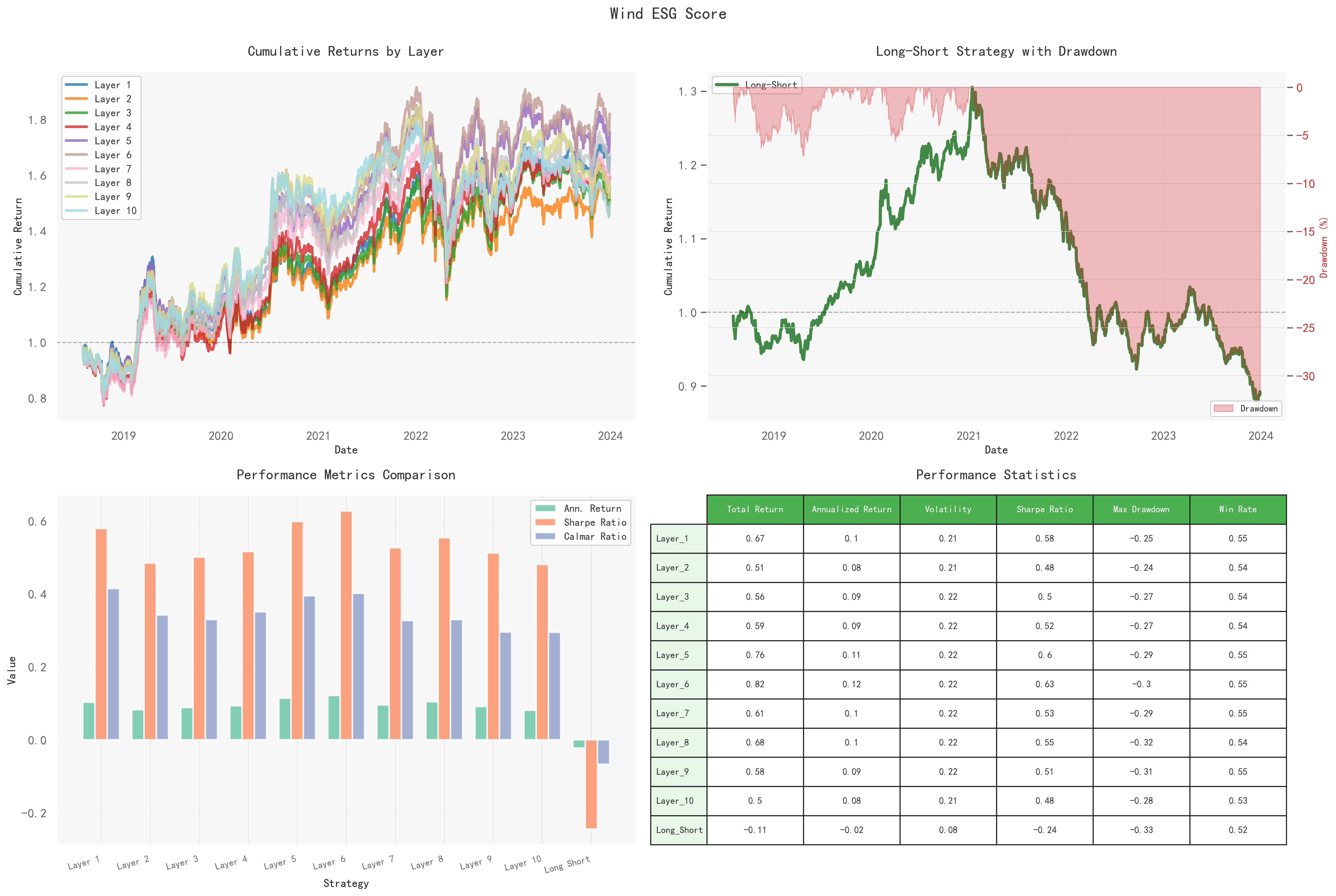 分层差异有限,层间交叉多;单调性不成立。
我们看到多空收益图:
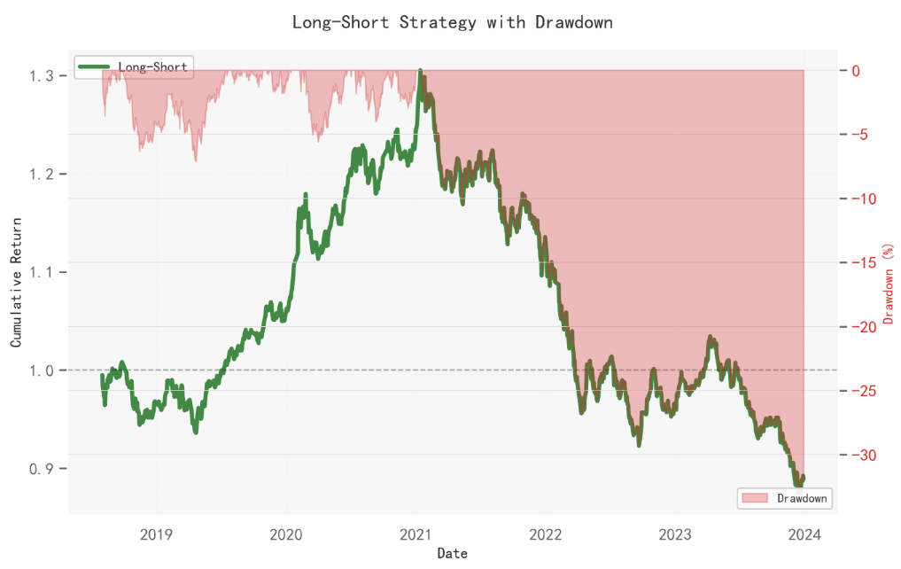
该策略覆盖期较短,经历一段“2019–2021 上行后便进入“2022–2023 回撤”的大周期;阶段性有效,随后熄火。
那ESG高的企业是一点都没用了吗?
| 层数 | 总收益 | 年化收益 | 波动率 | 夏普比 | 最大回撤 | 胜率 |
|---|---|---|---|---|---|---|
| 1 | 0.67 | 0.1 | 0.21 | 0.58 | -0.25 | 0.55 |
| 2 | 0.51 | 0.08 | 0.21 | 0.48 | -0.24 | 0.54 |
| 3 | 0.56 | 0.09 | 0.22 | 0.5 | -0.27 | 0.54 |
| 4 | 0.59 | 0.09 | 0.22 | 0.52 | -0.27 | 0.54 |
| 5 | 0.76 | 0.11 | 0.22 | 0.6 | -0.29 | 0.55 |
| 6 | 0.82 | 0.12 | 0.22 | 0.63 | -0.3 | 0.55 |
| 7 | 0.61 | 0.1 | 0.22 | 0.53 | -0.29 | 0.55 |
| 8 | 0.68 | 0.1 | 0.22 | 0.55 | -0.32 | 0.54 |
| 9 | 0.58 | 0.09 | 0.22 | 0.51 | -0.31 | 0.55 |
| 10 | 0.5 | 0.08 | 0.21 | 0.48 | -0.28 | 0.53 |
| 多空 | -0.11 | -0.02 | 0.08 | -0.24 | -0.33 | 0.52 |
答案是否定的,根据回测的最终结果我们可以看到:尽管第十层ESG高组别的股票年化收益最低,但其最大回撤也处于一个相对低值。
高ESG股票属于一个避风港的类型,它带来的收益不多但也不会亏损太多。
4.华证数据多维分析
接下来,我们通过调用上文已经编写好的函数,来对华证ESG数据的总分以及各个单项进行分层回测测试:
huazheng_esg_data = pd.read_parquet('hz_esg.parquet')

print("准备日线收益率数据")
daily_returns = prepare_daily_returns(daily_data)

# 华政ESG 4个分层回测
huazheng_scores = [
    ('综合得分', '综合得分'),
    ('E得分', 'E得分'),
    ('S得分', 'S得分'),
    ('G得分', 'G得分')
]

for score_name, score_col in huazheng_scores:
    print(f"\n" + "="*80)
    print(f"华政{score_name}回测")
    print("="*80)

    # 预处理数据
    esg_huazheng = preprocess_esg_data(huazheng_esg_data, score_column=score_col)

    # 分层(使用统一函数)
    esg_huazheng_classified = classify_score_per_period(esg_huazheng, score_col,
                                                        n_layers=10, data_source=f'华政{score_name}')

    # 扩展到日线
    daily_with_huazheng = expand_to_daily_with_t1(esg_huazheng_classified, daily_returns)

    # 清洗
    daily_with_huazheng = daily_with_huazheng.replace([np.inf, -np.inf], np.nan)
    daily_with_huazheng = daily_with_huazheng[daily_with_huazheng['return'].between(-0.5, 0.5)]
    print(f"[INFO] 清洗后华政{score_name}数据:{len(daily_with_huazheng):,} 条记录")

    # 回测
    huazheng_results = backtest_hold_between_events(daily_with_huazheng, min_names_per_layer_day=10)

    print(f"\n华政{score_name}回测结果:")
    print(pd.DataFrame(huazheng_results['statistics']).T.to_string())

    # 保存结果
    all_results[f'华政{score_name}'] = huazheng_results

    # 绘图
    plot_backtest_results(huazheng_results, title=f'Huazheng_{score_name}')


    print(f"[OK] 华政{score_name}多空策略报告已生成")

    generate_quantstats_report(
        huazheng_results['long_short_returns'],
        output_file=f'{report_dir}/huazheng_{score_name}_longshort_report.html',
        title=f'华政{score_name}多空策略报告'
    )
华证提供了更多的评级数据,包括单独的E,S和G评分,因此我们可以绘制四幅分层收益分析图:
4.1华证综合得分
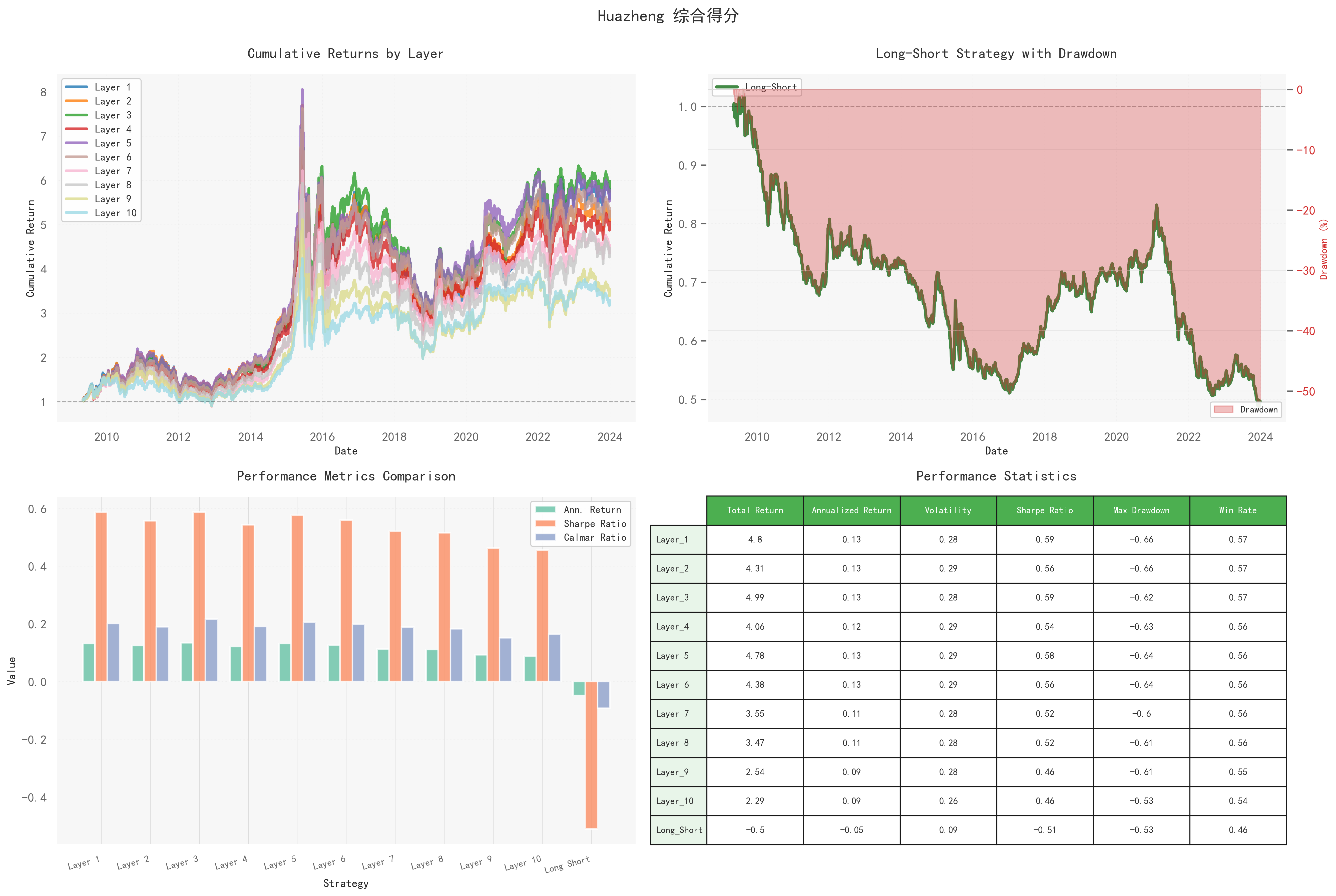
各分层净值走势高度同步,未呈现显著的单调递增特征,即ESG得分越高并不意味着收益越高。
在2014–2015年的市场泡沫期中,所有分层同步上涨后随之回落,说明该指标更多反映市场整体风格或周期波动,而非独立的超额收益来源。
多空组合(做多高分、做空低分)净值长期下行,累计回撤接近50%,年化收益约为-0.05,夏普比率为负,表明该策略在样本期内无效
从绩效指标来看,各分层年化收益介于0.09–0.13之间,夏普比率集中在0.5–0.6,显示出一定的防守稳定性。
4.2华证E评分
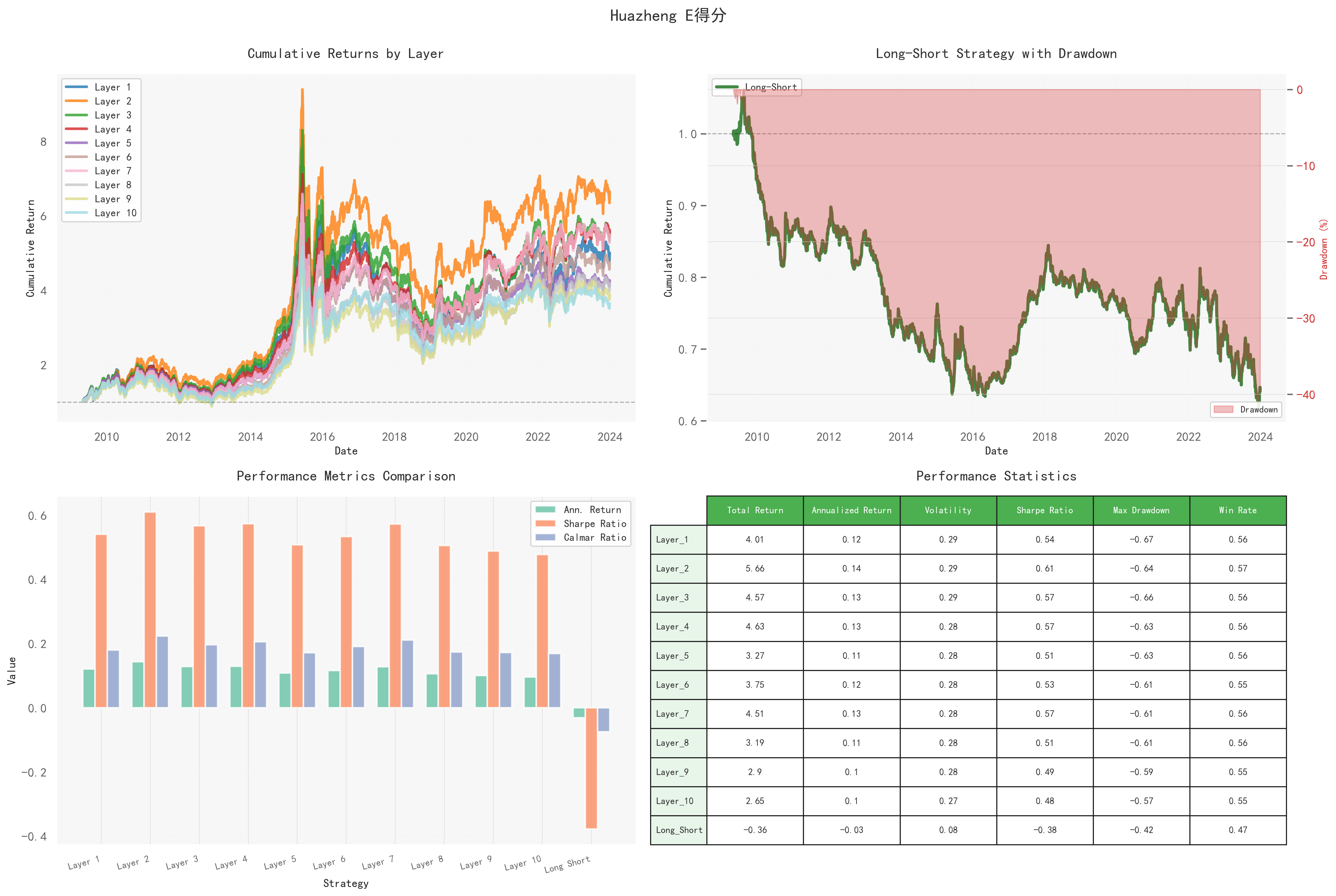
E评分在各分层间略有区分,但仍未形成稳定的单调关系,仅有个别中高分组合在特定阶段表现略优。
多空净值从初期即持续走弱,年化收益约为-0.03,夏普比率为负。各分层波动率介于0.27–0.29,回撤幅度也较为接近。
结果表明:环境评分的影响更多依赖政策或行业景气窗口,并不具备持续的超额收益能力。
4.3华证S评分
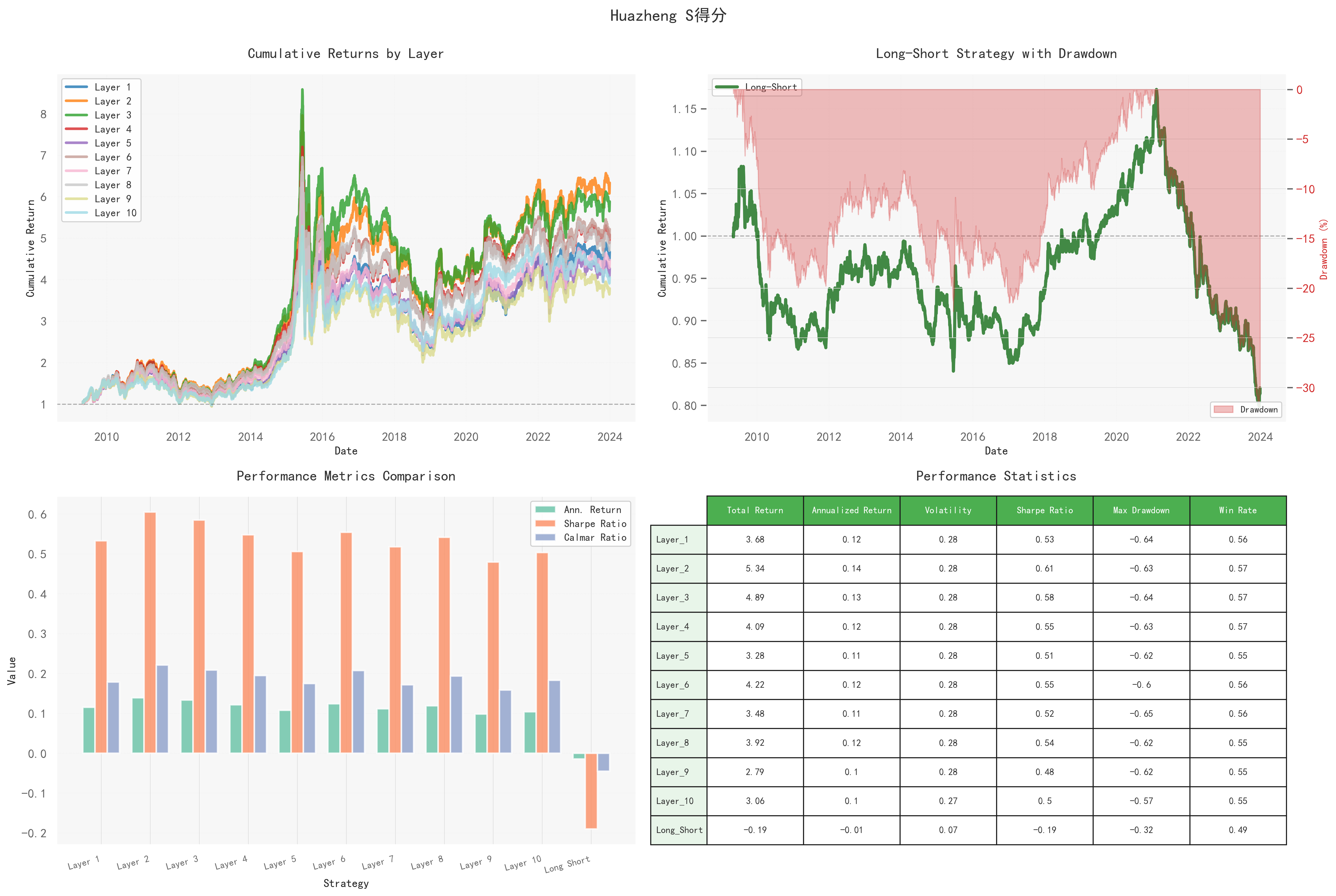
社会评分各分层净值依然高度同步,中段分层偶尔表现更优,但整体排序不稳定。
多空策略收益长期小幅为负,年化约-0.01,且回撤幅度较深,说明“做多高社会评分、做空低社会评分”的策略不具备盈利基础。
整体绩效与综合评分及E评分接近,防御属性虽略弱于G评分,但相较于无筛选基准仍有一定优势,不过效果有限。
4.4华证G评分
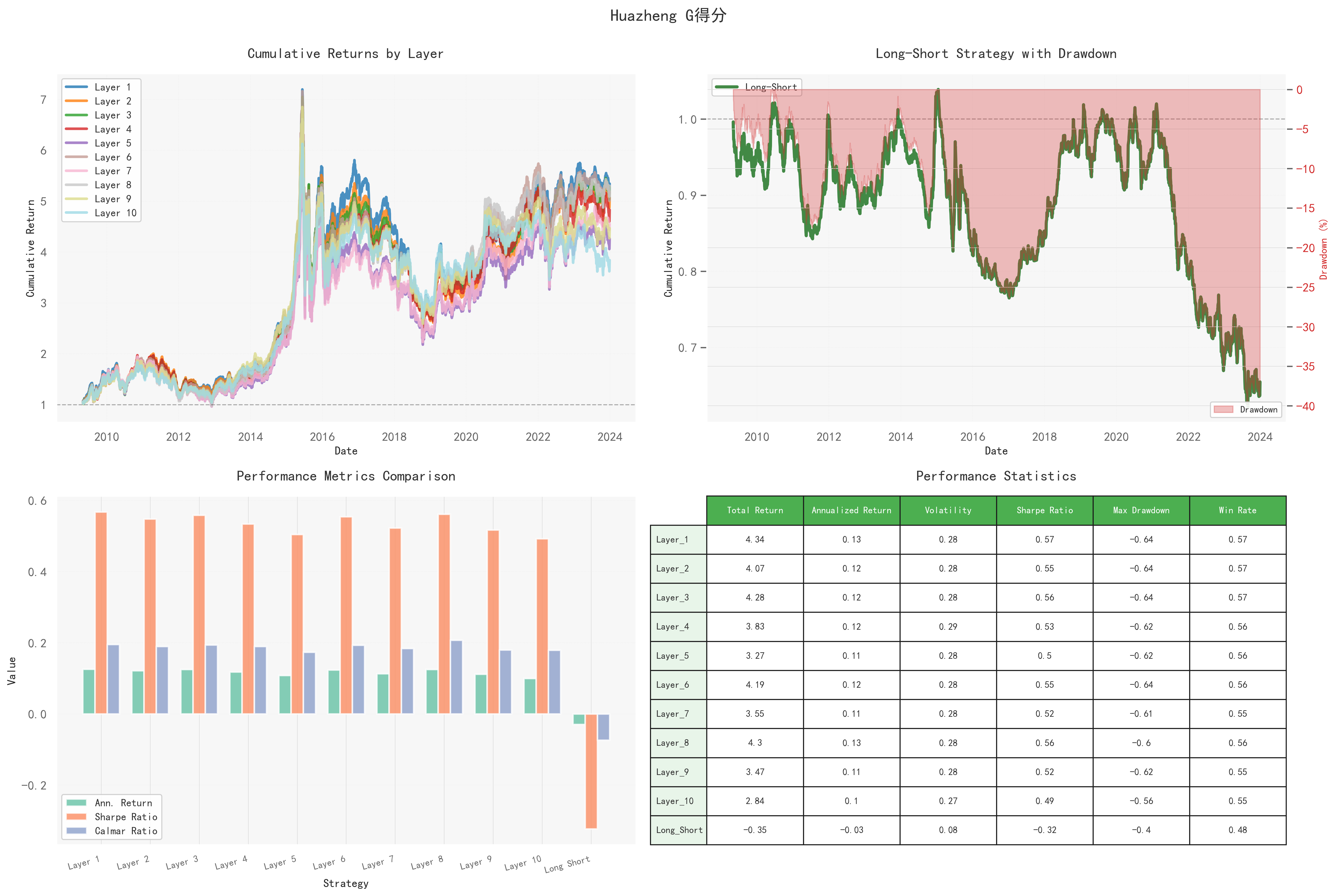
治理评分同样未呈现稳定的单调收益关系,其波动与回撤控制在此四类评分中最为规整,显示出类似低波因子的特征。
多空净值持续下行,年化收益约-0.03,夏普比率为负,印证了“做多好治理、做空差治理”的策略并不能穿越周期。
该评分主要体现出低波动+低回撤的风险控制特性,更适合作为组合中的风险缓冲单元,而非进攻性信号。
5综合比较
五张图给出同一个答案:ESG 分层不产生稳定的收益排序,多空长期为负;但高分层普遍更“稳”,回撤与波动更低。可以作为风险约束以及低波权重。
如需获取完整代码,可以订阅「Quantide Research」平台会员。平台介绍及付费方式https://mp.weixin.qq.com/s/j1r-cH_3Agc7fz1WwGrYFQ