涨到溢出！PEPE告诉我，大盘还能涨几多？

这两天涨得喜气洋洋的，不过，对东财的程序小哥哥来说，可能还得加班了，因为涨得太好，程序溢出了：

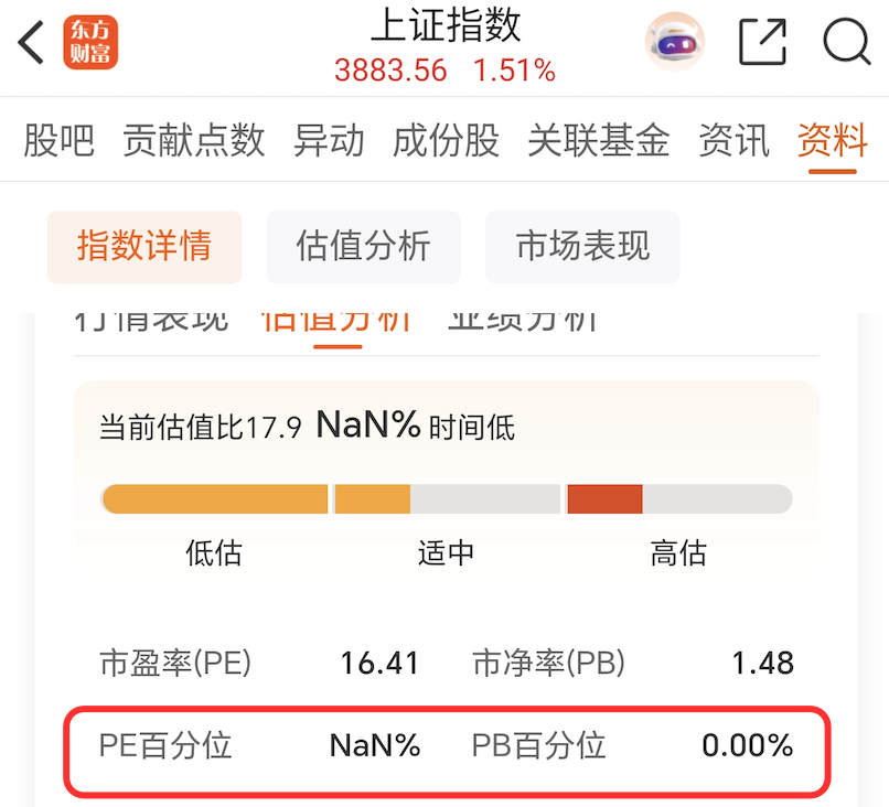
这是什么情况？

温故而知新

在2024年9月，我们曾发表《节前迎来揪心一幕！谁来告诉我，A股现在有没有低估？》一文。在那篇文章中，我们使用了akshare获取了上证指数的市盈率数据，并通过分位数和趋势分析，探讨了当时A股市场的估值情况。

当时我们的结论是：

如果仅从分位数统计来看，当下的A股是低估的。但如果考虑到市盈率总体上一直处在上升的趋势，以及最近一年来PE与指数涨跌的背离情况，判断A股是否已经低估还存有疑问，应该纳入更多维度进行判断。

现在是2025年8月，差不多快一年了。从成交量来看，市场似乎进入了狂飙期。我们去年使用过的技巧，是否还能用来预测未来的走势呢？

还是让数据说话。

使用 Tushare 获取指数市盈率

Tushare上周给我们放了一个假。不过，还好现在已经恢复了。要获取指数的市盈率，我们需要用到函数index_dailybasic。

import pandas as pd
import matplotlib.pyplot as plt
import matplotlib.dates as mdates
from datetime import datetime

pro = pro_api()

def get_index_pe_close(ts_code='000001.SH', start_date='20100101', end_date='20250825'):
    # 获取指数PE数据
    df_pe = pro.index_dailybasic(ts_code=ts_code, 
                                start_date=start_date, 
                                end_date=end_date, 
                                fields='trade_date,pe_ttm')
    df_pe.rename(columns={'trade_date': 'date', 'pe_ttm': 'pe'}, inplace=True)
    df_pe['date'] = pd.to_datetime(df_pe['date'])
    df_pe.set_index('date', inplace=True)
    
    # 获取指数收盘价数据
    df_price = pro.index_daily(ts_code=ts_code,
                              start_date=start_date,
                              end_date=end_date,
                              fields='trade_date,close')
    df_price.rename(columns={'trade_date': 'date'}, inplace=True)
    df_price['date'] = pd.to_datetime(df_price['date'])
    df_price.set_index('date', inplace=True)
    
    # 合并数据
    df = df_pe.merge(df_price, left_index=True, right_index=True, how='inner')
    
    # 排序
    df.sort_index(inplace=True)
    
    # 移除PE为空的记录
    df = df.dropna(subset=['pe'])
    
    return df

得到 pe 数据之后，让我们先来看一下直观走势：

# 绘制PE走势图
fig, ax = plt.subplots(figsize=(12,6))

color = "tab:red"
ax.plot(df.index, df["pe"], label="PE", color=color)
ax.set_xlabel("Year")
ax.set_ylabel("PE", color=color)
ax.xaxis.set_major_locator(mdates.YearLocator())
ax.xaxis.set_major_formatter(mdates.DateFormatter('%Y'))

df = get_index_pe_close(start_date="20100101")

# 添加分位数线
for i in range(1, 4):
    quantile = df["pe"].quantile(i/4)
    ax.axhline(quantile, color='gray', linestyle='--', label=f"{i/4:02.0%}")

plt.title("SSE Index PE Ratio (via Tushare)")
plt.legend(loc="upper left")
plt.grid(True)
plt.show()

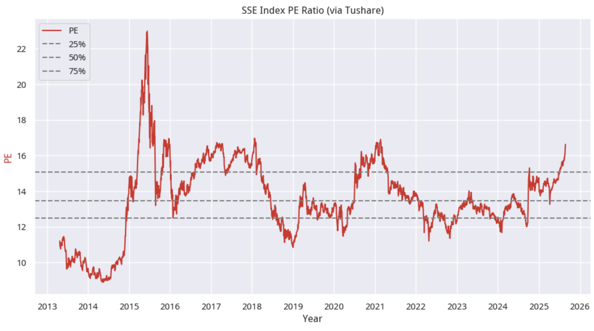
数据表明，如果我们忽略2015年那段癫狂的历史（场外融资加杠杆），那么现在的 PE 水平已经是相当高了。

到底有多高呢？

def show_pe_quantile(df):
    # 计算当前PE分位数
    current_pe = df['pe'].iloc[-1]
    rank = df['pe'].rank().iloc[-1]
    percentile = rank / len(df)
    print(f"当前PE分位: {percentile:.2%}")

show_pe_quantile(df)

df = df[df.index > '2016-01-01']
show_pe_quantile(df)

如果从2013年起（tushare 似乎没有更早的数据了）开始算，那么当前PE分位数为95.18%；如果从2016年1月起算，那么当前 PE 分位数则已达到98.81%，很快就要满分了。作为指数来讲，确实是有点高了。

当前的 PE 值，是多少天以来的最高值呢？通过 pandas 可以很容易计算出来：

def find_days_since_max_pe(df):
    """计算当前的PE是过去多少天以来的最大值"""
    if df.empty or len(df) < 2:
        return None
    
    # 获取当前PE值
    current_pe = df['pe'].iloc[-1]
    
    # 找到当前PE值在历史数据中的最大值位置
    max_pe_idx = df['pe'].idxmax()
    
    # 计算距离最大值日期的天数
    current_date = df.index[-1]
    days_since_max = (current_date - max_pe_idx).days
    
    return days_since_max, max_pe_idx

find_days_since_max_pe(df)

答案是，现在的 PE 值是2018年1月24日以来的最大值，也就是创了7年来的新高。

假设指数能稳住，那么能让 PE 回到安全区的惟一答案，就是要靠企业利润增长了。如果指数就停在这个位置，要让 PE 回到安全区，需要企业利润增加多少呢？

我们通过下面的方法来计算：

def required_earnings_growth(df, target_percentile=0.75, target_index=None):
    """计算使PE分位数降到目标值所需的盈利增长百分比"""
    if df.empty:
        return None
    
    # 获取当前PE值和当前指数点位
    current_pe = df['pe'].iloc[-1]
    current_index = df['close'].iloc[-1]
    
    # 如果指定了目标指数点位，则计算在该点位下的目标PE值；否则使用数据框中目标分位数对应的PE值
    if target_index is not None:
        # 根据PE = Price / Earnings，计算目标指数点位下的PE值
        # 假设盈利不变，目标PE = target_index / (current_index / current_pe)
        # 即 target_pe = target_index * current_pe / current_index
        current_pe = target_index * current_pe / current_index


    # 计算目标PE值（目标分位数对应的PE）
    target_pe = df['pe'].quantile(target_percentile)
    
    # 如果当前PE已经低于目标PE，则不需要盈利增长
    if current_pe <= target_pe:
        return 0.0
    
    # 计算所需盈利增长百分比
    # PE = Price / Earnings => Earnings = Price / PE
    # 要使PE从current_pe降到target_pe，需要:
    # (Price / target_pe) / (Price / current_pe) - 1 = current_pe / target_pe - 1
    required_growth = (current_pe / target_pe) - 1
    
    return required_growth

required_earnings_growth(df)

通过计算可知，在现有的指数上，如果要让 PE 回到75%分位以下，那么企业利润需要增加10.2%。如果要让 PE 回到84.13%分位（即一个标准差）以下，那么企业盈利需要增长5.5%。根据企业的年利润增长水平，我们大致可以估算出这需要多少年。当然，这要求企业的年利润增长水平必须是正的。

如果我们希望指数能上涨到4000点，PE 还要回到一个标准差以下，那么企业利润必须增长8.68%以上。

情况就是这么个情况。总之，我们已经进入了『无人区』，没有数据可以利用了。

本文代码可以匡醍研究平台运行和下载。